This post will cover how I solved the circuit and follow-on algebra problems for the pi-pad calculator and its resistor values. I am curious to know what the best way to solve this problem is today with modern analysis tools. Hopefully that will appear in a follow-up post soon!
I used good old-fashioned hand calculations with pencil and paper. How I had missed these from my university days. I don’t know that it’s particularly valuable for me to walk through all the algebraic steps. However, I will show my approach and my paper receipts should one want to follow along.
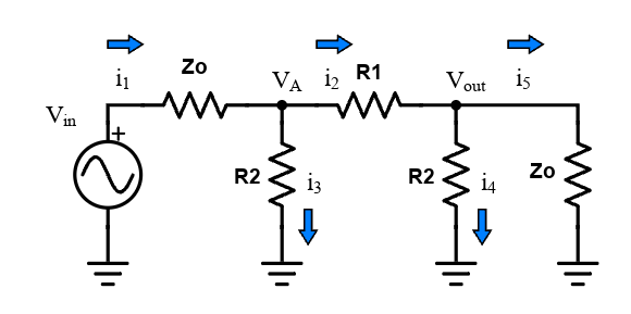
The first step was to create a schematic of the circuit and get clear about the problem that is being solved. When creating the pi-pad schematic for analysis, it is important to model \(Z_o\) resistive elements for source and load impedances. Of course a real RF source will not dissipate power through a series \(Z_o\) resistor; here it is simply used to define the constraint for input and output impedance being equivalent to source and load impedance. The actual RF attenuator circuit will ignore the series source resistor, \(Z_o\), and assume all power from \(V_in\) gets to the attenuator. Mismatch loss is ignored since we are targetting a perfect match and it is trivial to achieve excellent return loss. Once the schematic is drawn, it becomes a very straightforward nodal analysis problem like you might find in an introductory circuit analysis class.
Figure 1: Pi-Pad Schematic
I focused on the most common application of the attenuator circuit by assuming an equal source and load impedance. I have not personally used attenuators that transform source and load impedances, but perhaps that could be an interesting addition for the future at some point.
Solving the Nodal Analysis Problem
Figure 1 shows I have an arbitrary \(V_{in}\) node, and two voltage nodes \(V_A\) and \(V_{out}\) to solve for. I also label the currents associated with the different paths.
I then write the equations defining all the currents by inspection.
Then I plug in the current values in terms of \(V\) and \(R\) for the two current summation equations and simplify. If you would like to follow along with the steps to derive the final form of the nodal analysis equations, they are shown in the dropdown below.
Hand Calculations
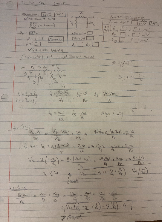
Here’s the original hand calculations along with the hand-drawn original concept for the calculator project. Note that I’ve swapped the reference designators on the resistor to match the published calculator and Figure 1 (\(R_1 = R_B\) and \(R_2 = R_A\)).
Figure 2: Concept and Nodal Analysis
After the fun times associated with algebraic manipulation, I come up with these equations: \[
\begin{equation}
0 = V_A \left(\frac{1}{R_1} \right) - V_{out} \left(\frac{1}{R_2} + \frac{1}{R_1} + \frac{1}{Z_o}\right) \label{eq:world}
\end{equation}
\tag{1}\]
These equations provided the foundation to implement the simple solution in Python used in the calculator tool. I assumed that the matrix multiplication method is the easiest way to solve a system of equations, so I look up how to do this in numpy and I incorporate it into my function.
Code
def solve_attenuation(self): z0 =self.z0 r1 =self.r1 r2 =self.r2ifself.use_standard_values: r1, r2 = get_standard_values(r1, r2, self.res_tol)# solve systems of equations v1_term_1 =1+ z0/r2 + z0/r1 vout_term_1 =-z0/r1 v1_term_2 =-1/r1 vout_term_2 =1/r1 +1/r2 +1/z0 vin =1 voltage_coefficients = [[v1_term_1, vout_term_1], [v1_term_2, vout_term_2]] A = np.array(voltage_coefficients) B = np.array([vin, 0]) X = np.linalg.solve(A, B) attenuation =round(-20*np.log10(2*X[1]/vin),2)self.outputs['attenuation'] = attenuationself.outputs['r1'] = r1self.outputs['r2'] = r2
Solving the Resistor Values
A few simple substitutions allow us to reduce to only two unknowns, \(R_1\) and \(R_2\). Before I got started simplifying the equations for \(R_1\) or \(R_2\), I replaced \(V_{out}\) with \(aV_A\) since I know I want to solve for attenution where \(a = \frac{V_{out}}{V_A}\).
First, I solved for \(R_2\) using Equation 1, which gave: \[
\begin{equation}
R_2 = \frac{aR_1}{1-a-a\frac{R_1}{Z_o}}
\end{equation}
\tag{3}\]
Then, I substituded \(R_2\) into Equation 2. Once again, if you’d like to follow the work for this derivation the details are shown in the dropdown below.
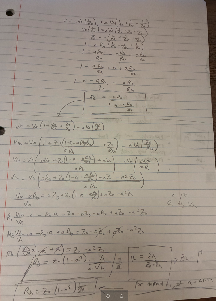
Solving for Resistors
Again, apologies for the reference designator switch (\(R_1 = R_B\) and \(R_2 = R_A\)).
For \(R_1\) I had to perform an additional substitution. Since we are solving for a perfectly matched attenuator, we want the input impedance equal to \(Z_o\), so we set \(V_A = \frac{1}{2}V_{in}\). Then using this substitution in Equation 4 we get: \[
\begin{equation}
R_1 = Z_o(1-a^2)\left(\frac{1}{2a}\right)
\end{equation}
\tag{5}\]
Now we find ourselves with a solution for \(R_1\) in terms of \(a\) and \(Z_o\) and an equation for \(R_2\) in terms of \(R_1\), \(a\), and \(Z_o\), so we are done.
Implementing the solution to solve for the resistor values in Python is straightforward. The only thing we really have to add is a conversion from the linear factor \(a\) (voltage gain) to attenuation in dB.
Code
def solve_resistors(self): z0 =self.z0# convert attenuation in dB to linear factor a a =10**(-self.attenuation/20)# delay rounding r1 to preserve floating point math r1 = z0*(1-a**2)/(2*a) r2 =round((a*r1) / (1- a - (a*r1/z0)),2) r1 =round(r1,2)ifself.use_standard_values: r1, r2 = get_standard_values(r1, r2, self.res_tol)self.outputs['r1'] = r1self.outputs['r2'] = r2self.outputs['attenuation'] =round(self.attenuation,2)
Solving Power Dissipation
Solving for power dissipation is quite simple after you already have all the circuit parameters.
I convert input power to an RMS voltage and calculate the output voltage from my attenuation factor \(a\). The voltage across the bridge resistor is simply the difference, and then I calculate power for all three using \(i^2R\).
Here is the power dissipation code from the calculator.